As R users, many, perhaps most, of us have had times where we’ve wanted our code to run faster. However, it’s not always clear how to accomplish this. A common approach is to rely on our intuitions, and on wisdom from the broader R community about speeding up R code. One drawback to this is it can lead to a focus on optimizing things that actually take a small proportion of the overall running time. Suppose you make a loop run 5 times faster. That sounds like a huge improvement, but if that loop only takes 10% of the total time, it’s still only a 8% speedup overall. Another drawback is that, although many of the commonly-held beliefs are true (for example, preallocating memory can speed things up), some are not (e.g., that apply functions are inherently faster than for loops). This can lead us to spend time doing “optimizations” that don’t really help. To make slow code faster, we need accurate information about what is making our code slow.

The profiler is a tool for helping you to understand how R spends its time. It provides a interactive graphical interface for visualizing data from Rprof, R’s built-in tool for collecting profiling data and, profvis, a tool for visualizing profiles from R. In this document, we’ll understand how to profile code using the profiler and walk through a couple examples to help diagnose and fix performance problems.

Getting started

Here’s an example of the profiler in use. We’ll create a scatter plot of the diamonds data set, which has about 54,000 rows, fit a linear model, and draw a line for the model. If you copy and paste this code into your R console, it’ll open the same profiler interface that you see in this document.

library(profvis)
profvis({
  data(diamonds, package = "ggplot2")

  plot(price ~ carat, data = diamonds)
  m <- lm(price ~ carat, data = diamonds)
  abline(m, col = "red")
})

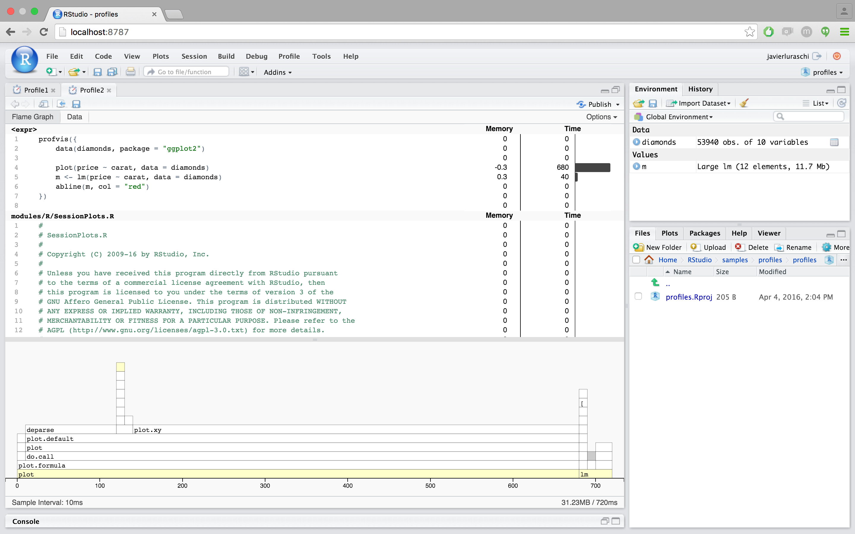
In the profiler interface, on the top is the code, and on the bottom is the flame graph. If the panels are too narrow, minimizing the console pane will help. In the flame graph, the horizontal direction represents time in milliseconds, and the vertical direction represents the call stack. Looking at the bottom-most items on the stack, almost 0.7 seconds are spent in plot, a much smaller amount of time is spent in lm, and almost no time at all is spent in abline – it doesn’t even show up on the flame graph.

Traveling up the stack, plot called plot.formula, which called do.call, and so on. Going up a few more levels, we can see that plot.defaultcalled a number of functions: first deparse, and later, plot.xy. Similarly, lm calls a number of different functions.

On the top, we can see the amount of time and memory spent on each line of code. This tells us, unsurprisingly, that most of the time is spent on the line with plot, and a little bit is spent on the line with lm.

Using the profiler

The profiler is composed by two main tabs:

• Flame graph
• Data

Using the flame graph view

The flame graph tab is interactive. You can try the following:

• As you mouse over the flame graph, information about each block will show in the info box.
• Yellow flame graph blocks have corresponding lines of code on the left. (White blocks represent code where profvis doesn’t have the source code – for example, in base R and in R packages. See the FAQ if you want package code to show up in the code panel.) If you mouse over a yellow block, the corresponding line of code will be highlighted. Note that the highlighted line of code is where the yellow function is calledfrom, not the content of that function.
• If you mouse over a line of code, all flame graph blocks that were called from that line will be highlighted.
• Click on a block or line of code to lock the current highlighting. Click on the background, or again on that same item to unlock the highlighting. Click on another item to lock on that item.
• Use the mouse scroll wheel or trackpad’s scroll gesture to zoom in or out in the x direction.
• Click and drag on the flame graph to pan up, down, left, right.
• Double-click on the background to zoom the x axis to its original extent.
• Double-click on a flamegraph block to zoom the x axis the width of that block.

Each block in the flame graph represents a call to a function, or possibly multiple calls to the same function. The width of the block is proportional to the amount of time spent in that function. When a function calls another function, another block is added on top of it in the flame graph.

The profiling data has some limitations: some internal R functions don’t show up in the flame graph, and it offers no insight into code that’s implemented in languages other than R (e.g. C, C++, or Fortran).

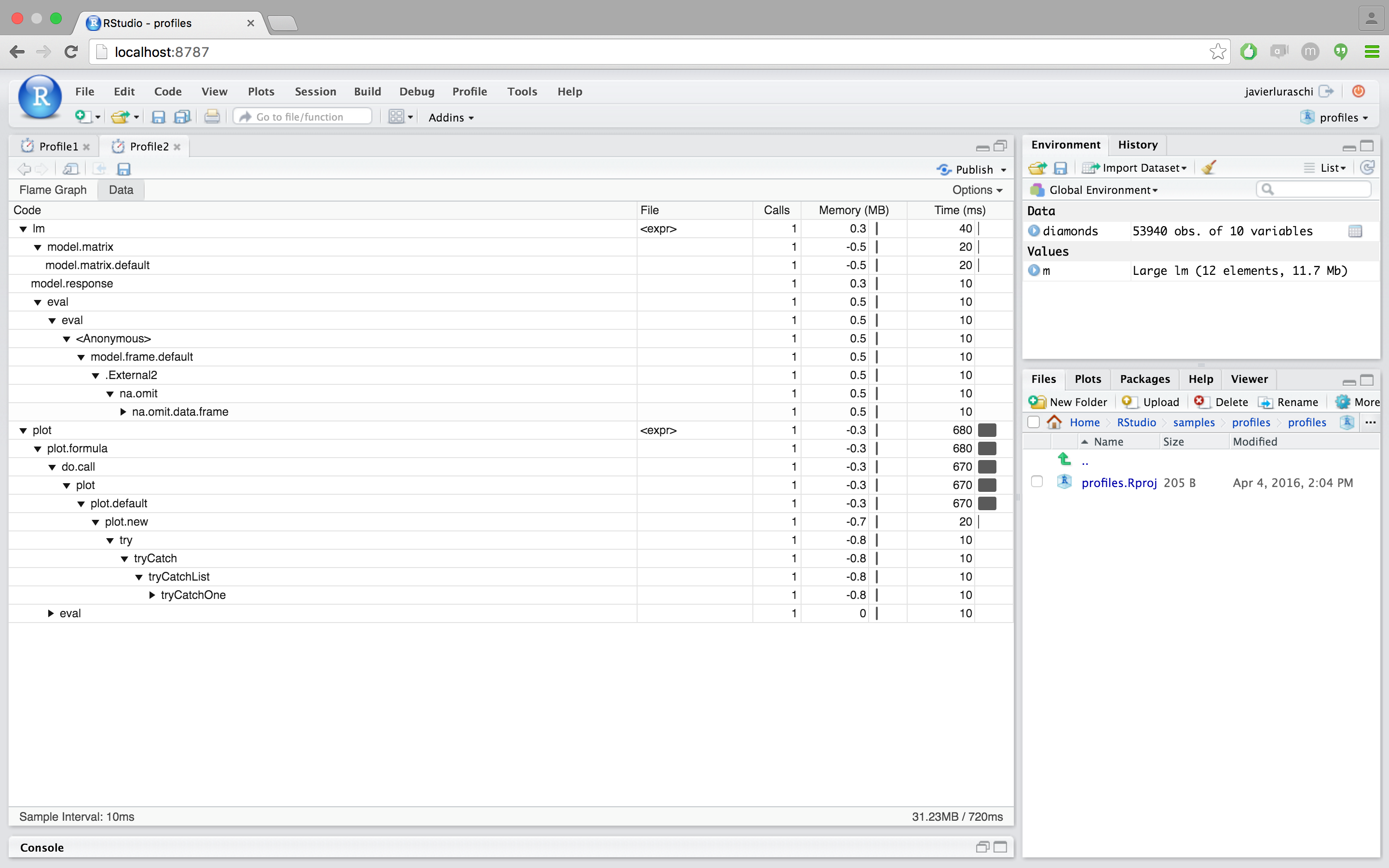
Using the data view

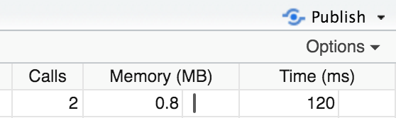
The data view provides a top-down tabular view of the profile. Click the `code` column to expand the call stack under investigation and the following columns to reason about resource allocation:

• Calls: This column represents the total number of calls performed. Even for fast calls, executing code several times can degrade performance and is worth investigating the total calls from this column is what you would expect to see.
• Memory: Memory allocated or deallocated (for negative numbers) at a give stack. This is represented in megabytes and aggregated over all the call stacks over the code in the given row.
• Time: Time spent in milliseconds. This field is also aggregated over all the call stacks executed over the code in the given row.

How profiling data is collected

The profiler usess data collected by Rprof, which is part of the base R distribution. At each time interval (default interval is 10ms), the profiler stops the R interpreter, looks at the current function call stack, and records the stack trace and memory into a file. Because it works by sampling, the result isn’t deterministic. Each time you profile your code, the result will be slightly different. Memory results are also influenced by the non-deterministic behavior of the garbage collector, which will make memory deallocations seem somewhat random.

Profiling examples

We’ll use the profiler to optimize some simple examples. Please keep in mind that R’s sampling profiler is non-deterministic, and that the code in these examples is run and profiled when this knitr document is executed, so the numeric timing values may not exactly match the text.

Profiling time

In this first example, we’ll work with a data frame that has 151 columns. One of the columns contains an ID, and the other 150 columns contain numeric values. What we will do is, for each numeric column, take the mean and subtract it from the column, so that the new mean value of the column is zero.

times <- 4e5
cols <- 150
data <-
 as.data.frame(x = matrix(rnorm(times * cols, mean = 5),
 ncol = cols))
data <- cbind(id = paste0("g", seq_len(times)), data)

profvis({
 # Store in another variable for this run
 data1 <- data

 # Get column means
 means <- apply(data1[, names(data1) != "id"], 2, mean)

 # Subtract mean from each column
 for (i in seq_along(means)) {
 data1[, names(data1) != "id"][, i] <-
 data1[, names(data1) != "id"][, i] - means[i]
 }
})

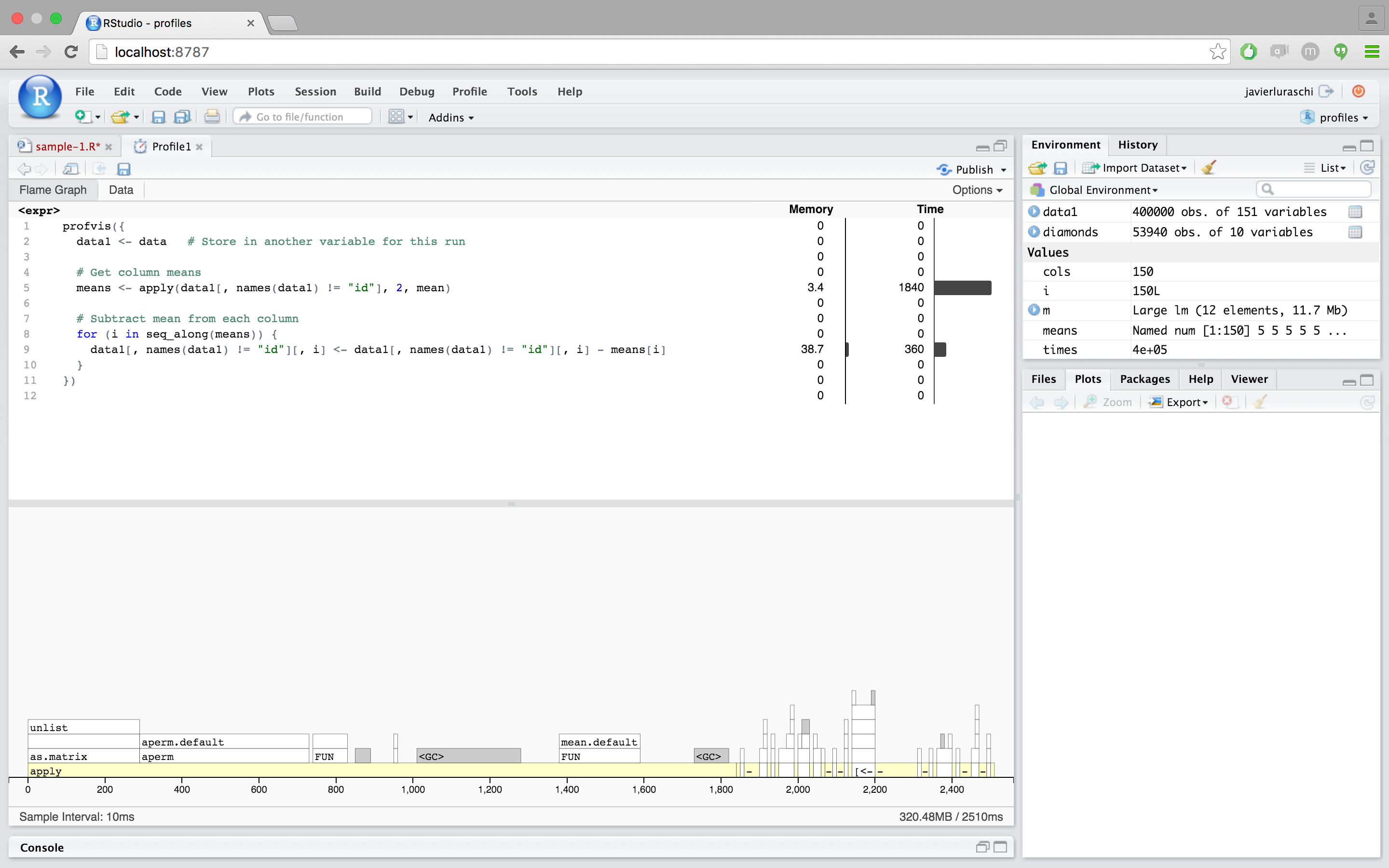
Most of the time is spent in the apply call, so that’s the best candidate for a first pass at optimization. apply calls as.matrix and aperm. These two functions convert the data frame to a matrix and transpose it – so even before we’ve done any useful computations, we’ve spent a large amount of time transforming the data.

We could try to speed this up in a number of ways. One possibility is that we could simply leave the data in matrix form (instead of putting it in a data frame in line 4). That would remove the need for the as.matrix call, but it would still require aperm to transpose the data. It would also lose the connection of each row to the id column, which is undesirable. In any case, using apply over columns looks like it will be expensive because of the call to aperm.

An obvious alternative is to use the colMeans function. But there’s also another possibility. Data frames are implemented as lists of vectors, where each column is one vector, so we could use lapply or vapply to apply the mean function over each column. Let’s compare the speed of these four different ways of getting column means.

profvis({
  data1 <- data
  # Four different ways of getting column means
  means <- apply(data1[, names(data1) != "id"], 2, mean)
  means <- colMeans(data1[, names(data1) != "id"])
  means <- lapply(data1[, names(data1) != "id"], mean)
  means <- vapply(data1[, names(data1) != "id"], mean, numeric(1))
})

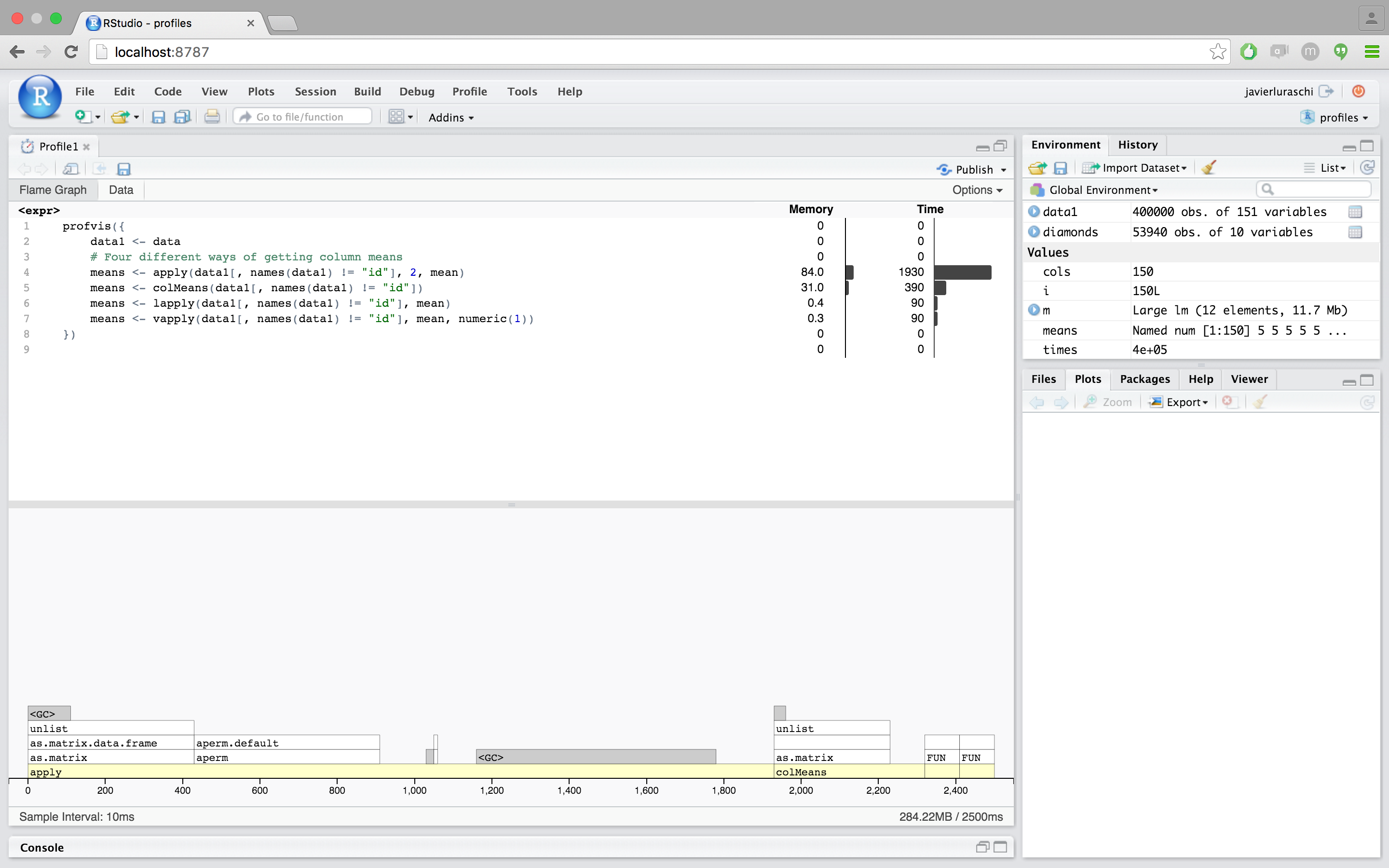
colMeans is about 6x faster than using apply with mean, but it looks like it’s still using as.matrix, which takes a significant amount of time.lapply/vapplyare faster yet – about 10x faster than apply. lapply returns the values in a list, while vapply returns the values in a numeric vector, which is the form that we want, so it looks like vapply is the way to go for this part.

(If you want finer-grained comparisons of code performance, you can use the microbenchmark package. There’s more information about microbenchmark in the profiling chapter of Hadley Wickham’s book, Advanced R.)

Let’s take the original code and replace apply with vapply:

profvis({
  data1 <- data
  means <- vapply(data1[, names(data1) != "id"], mean, numeric(1))

  for (i in seq_along(means)) {
    data1[, names(data1) != "id"][, i] <- data1[, names(data1) != "id"][, i] - means[i]
  }
})

Our code is about 3x faster than the original version. Most of the time is now spent on line 6, and the majority of that is in the [<- function. This is usually called with syntax x[i, j] <- y, which is equivalent to `[<-`(x, i, j, y). In addition to being slow, the code is ugly: on each side of the assignment operator we’re indexing into data1 twice with [.

In this case, it’s useful to take a step back and think about the broader problem. We want to normalize each column. Couldn’t we we apply a function over the columns that does both steps, taking the mean and subtracting it? Because a data frame is a list, and we want to assign a list of values into the data frame, we’ll need to use lapply.

profvis({
 data1 <- data
 
 # Given a column, normalize values and return them
 col_norm <- function(col) {
 col - mean(col)
 }
 
 # Apply the normalizer function over all columns except id
 data1[, names(data1) != "id"] <-
   lapply(data1[, names(data1) != "id"], col_norm)
})

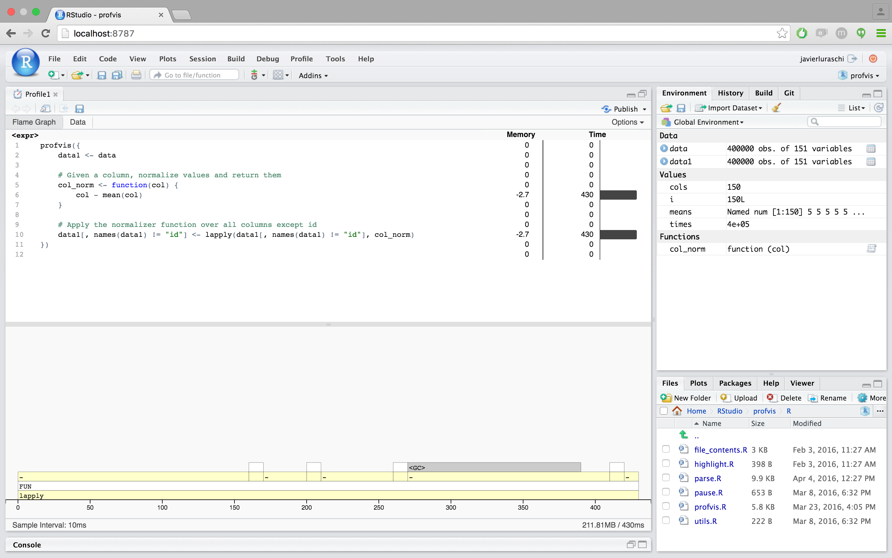
Now we have code that’s not only about 8x faster than our original – it’s shorter and more elegant as well. Not bad! The profiler data helped us to identify performance bottlenecks, and understanding of the underlying data structures allowed us to approach the problem in a more efficient way.

Could we further optimize the code? It seems unlikely, given that all the time is spent in functions that are implemented in C (mean and -). That doesn’t necessarily mean that there’s no room for improvement, but this is a good place to move on to the next example.

Profiling memory

This example addresses some more advanced issues. This time, it will be hard to directly see the causes of slowness, but we will be able to see some of their side-effects, most notably the side-effects from large amounts of memory allocation.

Suppose you have a data frame that contains a column for which you’d like to take a cumulative sum (and you don’t know about R’s built-in cumsumfunction). Here’s one way to do it:

profvis({
  data <- data.frame(value = runif(3e4))

  data$sum[1] <- data$value[1]
  for (i in seq(2, nrow(data))) {
    data$sum[i] <- data$sum[i-1] + data$value[i]
  }
})

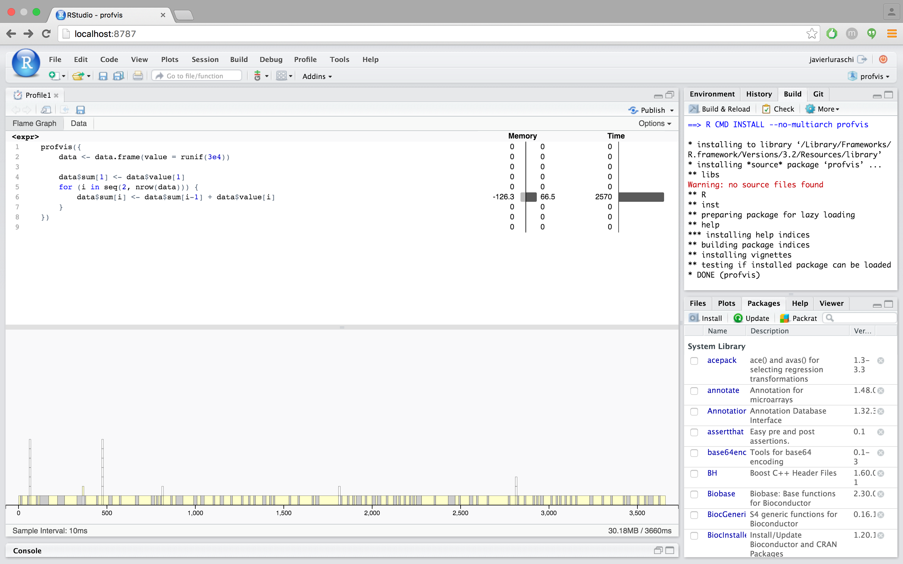
This takes over 2 seconds to calculate the cumulative sum of 30,000 items. That’s pretty slow for a computer program. Looking at the profvis visualization, we can see a number of notable features:

Almost all the time is spent in one line of code, line 6. Although this is just one line of code, many different functions that are called on that line.

In the flame graph, you’ll see that some of the flame graph blocks have the label $, which means that those samples were spent in the $ function for indexing into an object (in R, the expression x$y is equivalent to `$`(x, "y")).

Because $ is a generic function, it calls the corresponding method for the object, in this case $.data.frame. This function in turn calls [[, which calls [[.data.frame. (Zoom in to see this more clearly.)

Other flame graph cells have the label $<-. The usual syntax for calling this function is x$y <- z; this is equivalent to `$<-`(x, "y", z). (Assignment with indexing, as in x$y[i] <- z is actually a bit more complicated.)

Finally, many of the flame graph cells contain the entire expression from line 6. This can mean one of two things:

1. R is currently evaluating the expression but is not inside another function call.
2. R is in another function, but that function does not show up on the stack. (A number of R’s internal functions do not show up in the profiling data. See more about this in the FAQ.)

This profiling data tells us that much of the time is spent in $ and $<-. Maybe avoiding these functions entirely will speed things up. To do that, instead of operating on data frame columns, we can operate on temporary vectors. As it turns out, writing a function that takes a vector as input and returns a vector as output is not only convenient; it provides a natural way of creating temporary variables so that we can avoid calling $ and $<- in a loop.

profvis({
  csum <- function(x) {
    if (length(x) < 2) return(x)

    sum <- x[1]
    for (i in seq(2, length(x))) {
      sum[i] <- sum[i-1] + x[i]
    }
    sum
  }
  data$sum <- csum(data$value)
})

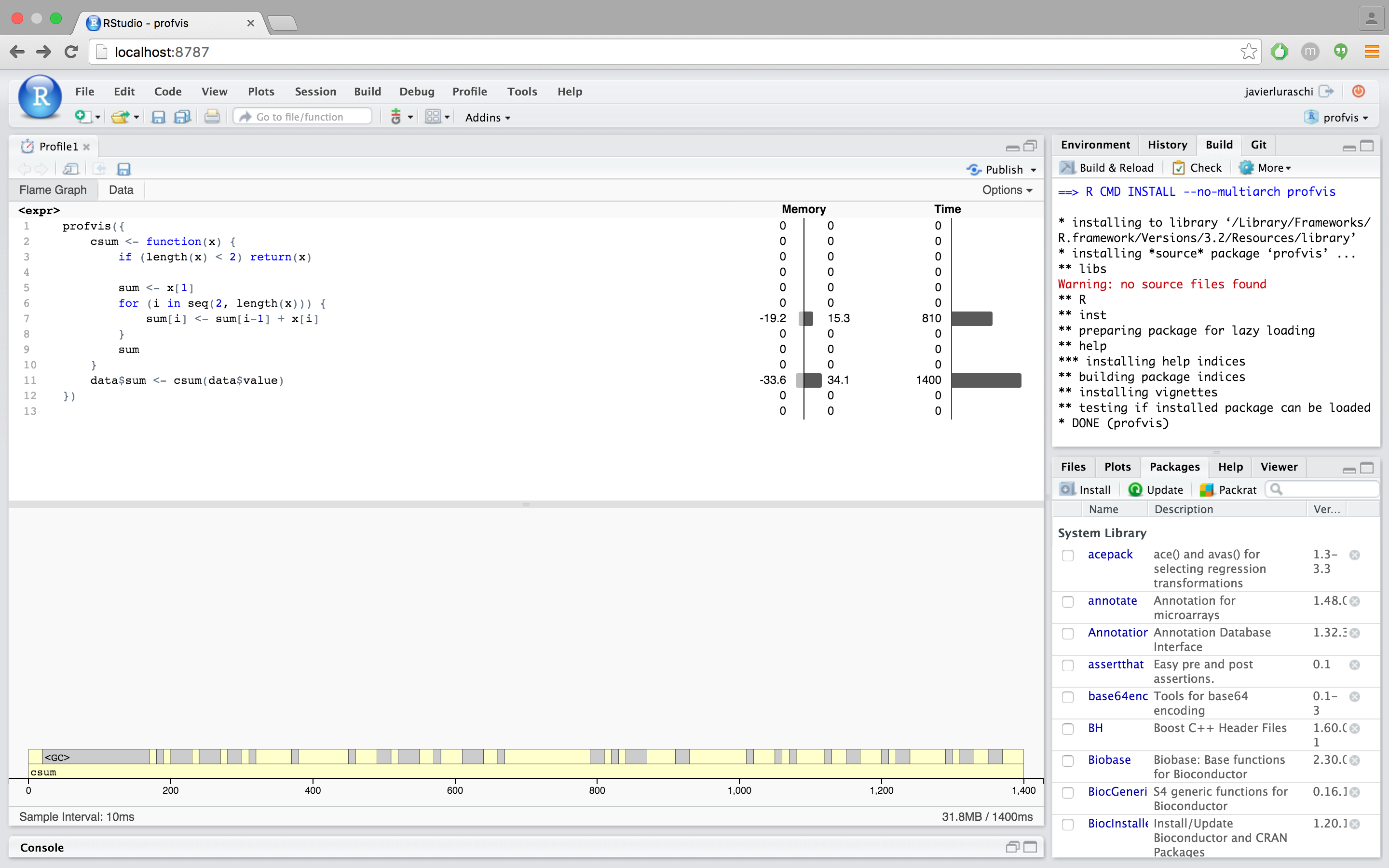
Using this csum function, it takes just over half a second, which is about 4x as fast as before.

It may appear that no functions are called from line 7, but that’s not quite true: that line also calls [, [<-, -, and +.

• The [ and [<- functions don’t appear in the flame graph. They are internal R functions which contain C code to handle indexing into atomic vectors, and are not dispatched to methods. (Contrast this with the first version of the code, where $ was dispatched to $.data.frame).
• The - and + functions can show up in a flame graph, but they are very fast so the sampling profiler may or may not happen to take a sample when they’re on the call stack.

You probably have noticed the gray blocks labeled <GC>. These represent times where R is doing garbage collection – that is, when it is freeing chunks of memory that were allocated but no longer needed. If R is spending a lot of time freeing memory, that suggests that R is also spending a lot of time allocating memory. This is another common source of slowness in R code.

In the csum function, sum starts as a length-1 vector, and then grows, in a loop, to be the same length as x. Every time a vector grows, R allocates a new block of memory for the new, larger vector, and then copies the contents over. The memory allocated for the old vector is no longer needed, and will later be garbage collected.

To avoid all that memory allocation, copying, and garbage collection, we can pre-allocate a correctly-sized vector for sum. For this data, that will result in 29,999 fewer allocations, copies, and deallocations.

profvis({
  csum2 <- function(x) {
    if (length(x) < 2) return(x)

    sum <- numeric(length(x))  # Preallocate
    sum[1] <- x[1]
    for (i in seq(2, length(x))) {
      sum[i] <- sum[i-1] + x[i]
    }
    sum
  }
  data$sum <- csum2(data$value)
})

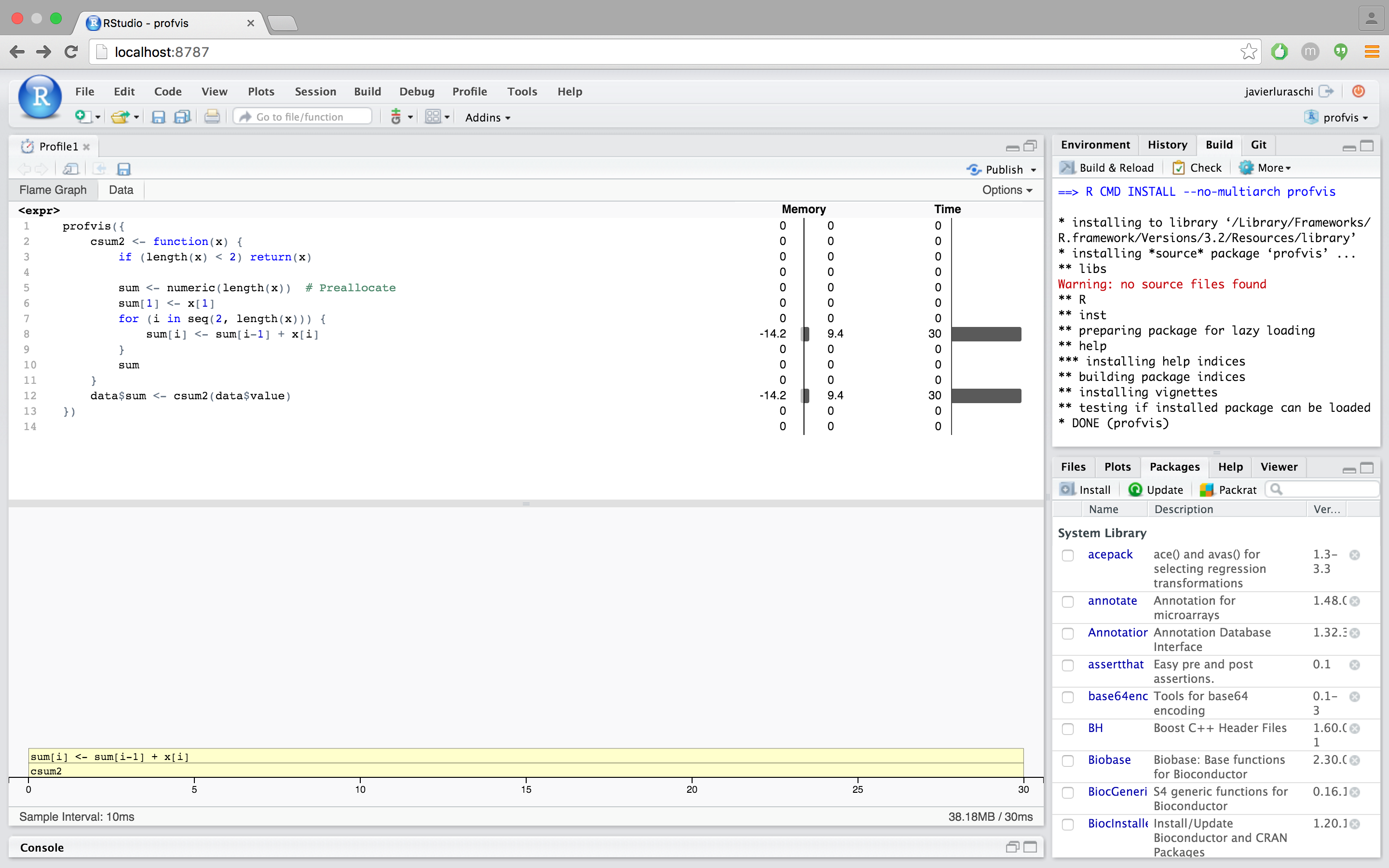
This version of the code, with csum2, is around 60x faster than our original code. These performance improvements were possible by avoiding calls to $ and $<-, and by avoiding unnecessary memory allocation and copying from growing a vector in a loop.

Frequently asked questions

Why do some function calls not show in the profiler?

As noted earlier, some of R’s built-in functions don’t show in the flame graph. These include functions like <-, [, and $. Although these functions can occupy a lot of time, they don’t show on the call stack. (In one of the examples above, $ does show on the call stack, but this is because it was dispatched to $.data.frame, as opposed to R’s internal C code, which is used for indexing into lists.)

In some cases the side-effects of these functions can be seen in the flamegraph. As we saw in the example above, using these functions in a loop led to many memory allocations, which led to garbage collections, or <GC> blocks in the flame graph.

How do I share a profile?

Right now the easiest way to do this is to generate the profile in RStudio, and publish to RPubs using the publish toolbar button:

What does <Anonymous> mean?

It’s not uncommon for R code to contain anonymous functions – that is, functions that aren’t named. These show up as <Anonymous> in the profiling data collected from Rprof.

Similarly, functions that are accessed with :: or $ will also appear as <Anonymous>. The form package::function() is a common way to explicitly use a namespace to find a function. The form x$fun() is a common way to call functions that are contained in a list, environment, reference class, or R6 object.

Those are equivalent to `::`(package, function) and `$`(x, "fun"), respectively. These calls return anonymous functions, and so R’s internal profiling code labels these as <Anonymous>. If you want labels in the profiler to have a different label, you can assign the value to a temporary variable (like adder2 above), and then invoke that.

Finally, if a function is passed to lapply, it will be show up as FUN in the flame graph. If we inspect the source code for lapply, it’s clear why: when a function is passed to lapply, the name used for the function inside of lapply is FUN.

How do I get code from an R package to show in the code panel?

In typical use, only code written by the user is shown in the code panel. (This is code for which source references are available.) Yellow blocks in the flame graph have corresponding lines of code in the code panel, and when moused over, the line of code will be highlighted. White blocks in the flame graph don’t have corresponding lines in the code panel. In most cases, the calls represented by the white blocks are to functions that are in base R and other packages.

The profiler can also show code that’s inside an R package. To do this, source refs for the package code must be available. There are two general ways to do this: you can install the package with source refs, or you can use devtools::load_all() to load a package from sources on disk.

Why does the flame graph hide some function calls for Shiny apps?

When profiling Shiny applications, the flame graph will hide many function calls by default. They’re hidden because they aren’t particularly informative for optimizing code, and they add visual complexity. This feature requires Shiny 0.12.2.9006 or greater.

Why does Sys.sleep() not show up in profiler data?

The R profiler doesn’t provide any data when R makes a system call. If, for example, you call Sys.sleep(5), the R process will pause for 5 seconds, but you probably won’t see any instances of Sys.sleep in the profiler visualization – it won’t even take any horizontal space. For these examples, we’ve used the pause function instead, which is part of the profvis package. It’s similar to Sys.sleep, except that it does show up in the profiling data.

Why is the call stack reversed for some of my code?

One of the unusual features of R as a programming language is that it has lazy evaluation of function arguments. If you pass an expression to a function, that expression won’t be evaluated until it’s actually used somewhere in that function.

Why does the profiler tell me the the wrong line is taking time?

In some cases, multi-line expressions will report that the first line of the expression is the one that takes all the time. In the example below, there are two for loops: one with curly braces, and one without. In the loop with curly braces, it reports that line 3, containing the pause is the one that takes all the time.

Additional resources

Profiling by Hadley Wickham

Introduction to profvis by Winston Chang